ASPIDE

Usage Example.

Installing

ASPIDE is a software developed in JAVA (requires Java vers 1.6) and it is available for the platforms Windows, Linux and Mac OS X.

Launch the Installer in order to install ASPIDE. On the installation phase you are required to have a working internet connection.

In the download page it is also available the jar package of ASPIDE that does not need an installation process.

Start

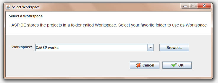
1. Select a workspace and then click OK.

When you start the program, the "Workspace Selector" dialog pops up. There you can select the workspace directory wher stores projects. In order to create a workspace in another directory click on the "Browse..." button and select the desired directory.
In the workspace directory all information about your projects, your preference settings, etc. will be stored.

2. Select the default executable path to execute your programs.

At the first start, you can choose the default executables paths for the solver used from application.
In particular you can choose the follows executables files:

DLV - used to execute simple DLV programs (DLV files);
DLV+ODBC - used to execute DLV programs with import/export features which load/store database tables;
DLV^DB - used to execute DLV programs by exploiting databases for import/export features and for mass memory execution;
DLV^E - used to execute DLV programs which exploits existential terms in rule heads;
IDPDraw - used to visualize the output of an ASP solver in an advanced graphical way;

DLT - used to execute advanced code templates;
Profiler - used to execute an prototypical profiler integrated in the application;
Spock - used to debug ground ASP programs;
ARVis - used to visualize Answer Sets and their releations by means of a directed graph.

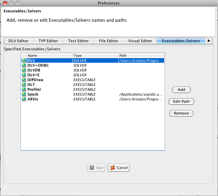
The default executables paths can be setted after by preferences wondows Window->Preferences.

3. The program starts and the start screen appears.

In the start screen there are a set of shortcuts to manipulate the workspace and the projects its contains.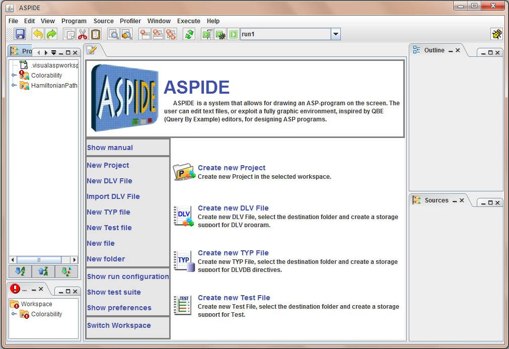

User Interface

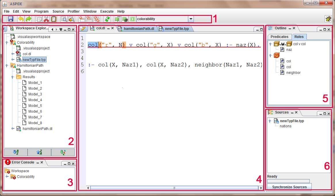
The user interface consists in a dynamic view composed from:

Toolbar men� - used to access the most important fueatures of application;
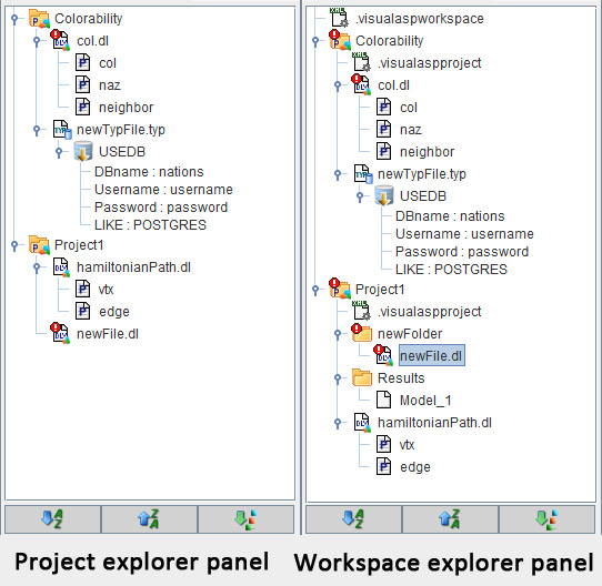
Explorer panels - there are two explorer panel: the Project Explorer that shows the projects and its files (DLV files, Typ files and Test files); the workspace explorer shows the content of project folder, showing the internal project files and the external files;
Error console - shows errors errors organized by project;
Edit area - where project files can be typed;
Outline - represents a program code overview which can be used to quickly access the respective lines of the code;
Sources navigation - shows the sources relating to a particular project.

Toolbar

The toolbar allows you to quickly handle files currently displayed in the text editor or running a project:

- saves the content of the current text editor;
- undo/redo commands;
- copy/cut/paste commands;
- find/find-next commands;
- close-current/close-others/close-all editors commands;
- switch text/visual command;
- start selected run configuration with profiler;
- start selected run configuration with debugger;
- execute selected run configuration;
- run configuration selector;

Explorer menu

ASPIDE provides two type of explorer panel, the Project Explorer Panel shows only the project folders and files (Dlv file, TYP file and test files).
The Workspace Explorer Panel have a higher level detail, showing the subfolders project and simple files present in the workspace.

Explorer popup menu

The explorer panels provide popup menu used to manage workspace and projects, using the right click on the panel, the user can access the functionality of creating, deleting and editing files and projects: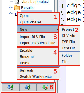

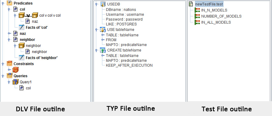
- open the selected file, in textual or visual mode;
- create new projects or files ;
- import and export dlv files from projects;
- modify selected object, rename, enable/disable or delete files and projects;
- refresh the explorer panel content;
- change the object order visualized in the explorer panel;

Outline view

ASPIDE creates an outline view which graphically represents program elements. Each item in the outline can be used to quickly access the corresponding line of code. The outline changes in relation of the file showed in the editor.

Sources panel

Another panel used in ASPIDE allows to visualize all sources create in a project.

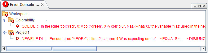
Error console

The system provides a console that stores all errors (syntactic and semantic errors) presents in the worwspace, organazing its for project and file membership.
A double click on visualized error open automatically the editor with the file that contains the error, signaling the affected code line.

Text editor

The editing of ASP files is simplified by an advanced text editor, which provides several functionalities, from the simple highlighting, to auto completion of predicates and variable names.

Text coloring

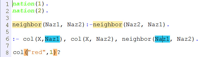
In the follow image is present an example of DLV file editor with all text coloring features:

At line 1 the predicate nation is green colored because the predicate nation is used in the project DB sources;
At line 4 is present an example of pair word highlighter that marks same words on the editor;
At line 6 is present an example of pair variable highlighter that marks same variables in a rule;
At line 8 is present an example of pair parenthesis highlighter that marks start and end of a parenthesization;
The editor marks with different colors keywords, strings and integers.

The colors showed in the previus image are the default colors, the user can change its by preferences dialog.

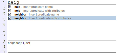
Auto completion

ASPIDE provides a functionality that suggest the user how to complete the portion of code he is writing, just during the typing. In the our system the automatic completion tool works on what has been declared by the programmer up to that time; in other words, it works on the list of atoms previously specified in the program (in the same file or in the other DLV files stored in the same project). The automatic completion suggests also the variables used in the same rule and the predicates used in the directives for database mapping. The auto-completion popup is showed pressing the ctrl + space key.

Error/Worning highlighter

When the user types a file, it is parsed by the parsing module and its syntactical correctness is verified. If an error is identified, the line that contains the error is signed on the text editor by a line. In the follow image are present an example of error highlighter (red line, signals an arity error of col predicate) and an example of warning highlighter (yellow line, signals the predicate neighbor is never used in head of a rule in this program).

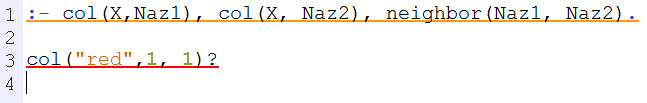
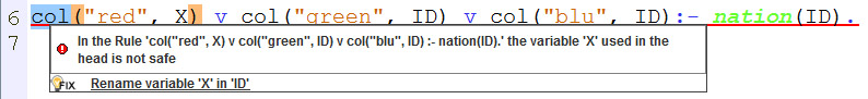
Quick fix

The dynamic errors highlighting is supported by a tool that provides solutions to correct the detected error. When you click on the piece of code which contains an error, the application shows a popup window containing a list of suggestions; the use of a quick fix, edits the code directly on the text editor. The follow figure is an example of quick-fix for unsafe rule, the popup panel shows the possible solutions to resolve the problem.

Visual Editor

The Visual Editor of ASPIDE allows for drawing ASP programs by exploiting a fully-graphical way. Using the Visual Editor, logic rules (facts, normal and disjunctive rules, constraints) can be defined using a QBE-like style, by making operations of projections, join, union and intersection.

This section shows a generic overview of the Visual Editor explaining the role of the single panels.
After that, the section shows how to use the Visual Editor by exploiting an example and drawing, step by step, the single rules.

Visual Editor overview

The figure 1 shows an overview of the Visual Editor.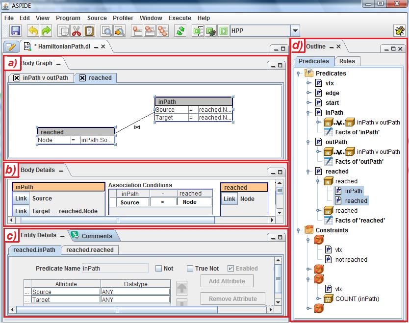

Figure 1. Overview of the Visual Editor.

In the figure, the section a is the Body Graph panel where the user can have a general view of the body of a rule. It is a graph representation of the literals inserted in the body of a rule and shows the associations (join, union, intersection, not) between the literals inserted in the body. Each literal is an Entity and it is represented, in this graph, as a rectangular shape. Inside each entity there are also the join conditions of the respective attributes between (i) the attributes of the same entity, (ii) the attributes of this entity with other entities of the body, and (iii) the attributes of this entity with the predicates of the head.

By selecting the entities of the Body Graph, the section b shows the details of the body. In particular we can see all the attributes belonging to the entities and we can do operations like join between attributes of the body and binding (unbinding) of the attributes with one or more attributes of the head. We can set also join conditions like equality/disequality of attributes with other attributes or constants.

The section c shows the details of single entities that we have selected. For each entity we can add, edit or delete attributes and set the datatypes. An entity can be also a rule, so we can use the same section to insert static values to the head of the rule, to give a name to a rule, to disable a rule, etc… If the entity selected is some literal of the body, with this section we can negate the literal of the rule and the same section will show which attributes (if any) are not safe.

The section d shows the outline of the program that we are building. We can view the program by Predicates or by Rules.
Using the view by Predicates the outline shows, using a tree visualization, the list of all predicates and, for each predicate, a list of rules that have that predicate in the head. With this view, the constraints and the weak constraints are grouped in separated nodes respect to the predicates.
Using the view by Rules the outline shows the set of all rules without the grouping.
In both views we can do a mouse double-click on the rules to open those rules in the Body Graph for editing.
To insert the facts to a predicate we have to use the view by Predicates, and to select the node Facts of ‘predicateName’ where predicateName is the name of the corresponding predicate. After the selecting, the Entity Details panel shows a table where we can insert, edit and delete facts.

Example Program

Hamiltonian Path Problem

To show how the Visual Editor works, it is proposed a program example that resolves the Hamiltonian Path problem.
We consider the well-known Hamiltonian Path problem: Given a finite directed graph G = (V,A) and a node a of this graph, does there exist a path in G starting at a and passing through each node in V exactly once? This is a classical NP-complete problem in graph theory. Suppose that the graph G is specified by using facts over predicates vtx (unary) and edge (binary), and the starting node a is specified by the predicate start (unary). The following program solves the problem:

% Facts
vtx(1). vtx(2). vtx(3). vtx(4). vtx(5).
edge(1, 2). edge(2, 3). edge(3, 4). edge(4, 5). edge(3, 2). edge(1, 3). edge(2, 4). edge(5, 1).
start(1).

% Guess arcs of the path
r1: inPath(X, Y) v outPath(X, Y) :- edge(X, Y).

% Auxiliary rules
r2: reached(X) :- inPath(Y, X), reached(Y).
r3: reached(X) :- start(X).

% Checking part: specify constraints on solution.

% All vertexes must be in the path.
r4: :- vtx(X), not reached(X).
% A Target Node of the path cannot be the start node.
r5: :- start(X), inPath(_, X).
% Each vertex in the path must have
% at most one incoming and one outgoing edge.
r6: :- vtx(X), 2 <= #count{Y : inPath(X, Y)}.
r7: :- vtx(X), 2 <= #count{Y : inPath(Y, X)}.

The disjunctive rule (r1) guesses a subset S of the arcs to be in the path, while the rest of the program checks whether S constitutes a Hamiltonian Path. Here, an auxiliary predicate reached is defined, which specifies the set of nodes which are reached from the starting node. In the checking part, the constraint r4 enforces that all nodes in the graph are reached in the subgraph induced by S. The constraint r5 ensures that a target node of the inPath predicate cannot be the start node, while the two constraints r6 and r7 ensure that the set of arcs S selected by inPath meets the following requirements, which any Hamiltonian Path must satisfy: (i) a vertex must have at most one incoming edge, and (ii) a vertex must have at most one outgoing edge.

Inserting Predicates and Facts

We start by adding the input predicates: vtx, edge and start. More in detail, to add a predicate to the program, we click on the Program menu and select New Predicate (fig. 2).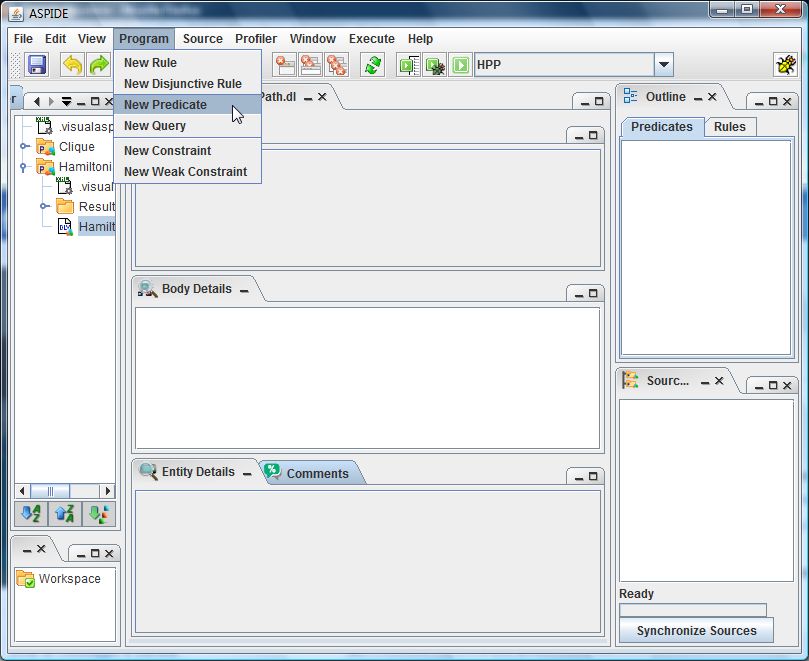

Figure 2. Creating a new Predicate

A dialog will ask for the name of the predicate to be inserted (fig. 3), and after specifying the required information and confirming the command, a new predicate icon appears on the Outline panel (fig. 4). In the panel placed in the bottom-center, labelled Entity Details (fig. 4), one can specify the arity of the predicate (currently selected in the Outline) by adding a number of attributes.

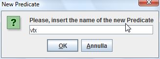
Figure 3. Entering a new predicate name

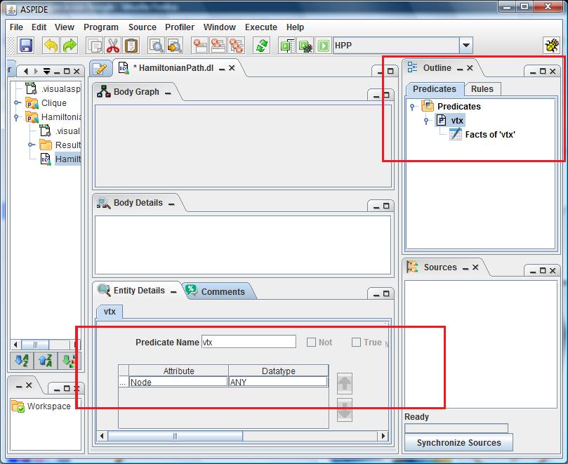
Figure 4. The predicate vtx in the Outline. Added the attribute Node in vtx

The system allows for specifying a name for each attribute, and a datatype. This additional information is very useful during the editing phase, since it allows for rapidly identifying and joining attributes.

In order to insert the facts to a predicate (e.g. vtx), we select Facts of vtx on the Outline panel, and the Entity Details panel will show a table when we can insert the facts of the predicate. Same actions to insert facts to the predicate edge (fig. 5).

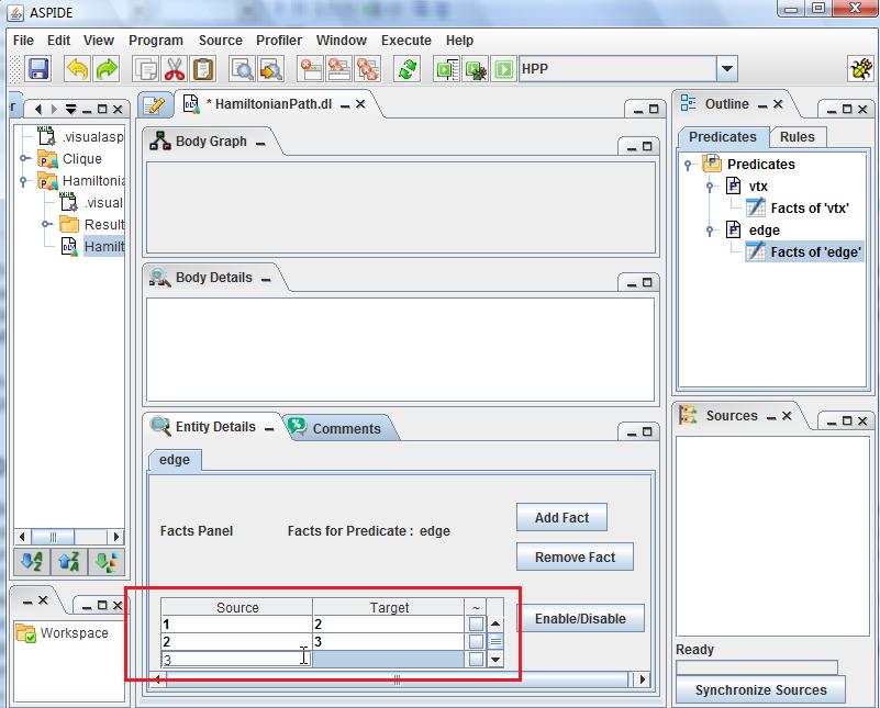
Figure 5. Inserting facts to the predicate edge

Drawing Rule r1

Now we insert the disjunctive rule r1 by selecting New Disjunctive Rule on the Program menu. The system opens a dialog window used to specify the head of the rule (fig. 6). In this window we can select predicates, that already exist and/or can type new predicates, to be added in head.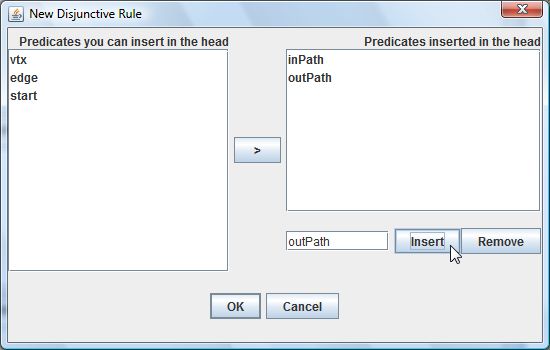

Figure 6. Dialog window for setting the head of the new disjunctive rule

We click on the OK button and the new disjunctive rule will be inserted to the Visual Editor both in the Outline and in the Body Graph panel situated on the top-center (fig. 7). Note that in the Outline we selected a visualization by predicates, so under both the predicates inPath and outPath the disjunctive rule is shown because it defines both the predicates. Then, one can specify its body by dragging predicates from the Outline panel to the Body Graph panel. In our example we drag the edge predicate in the body graph corresponding to our disjunctive rule (fig. 7).

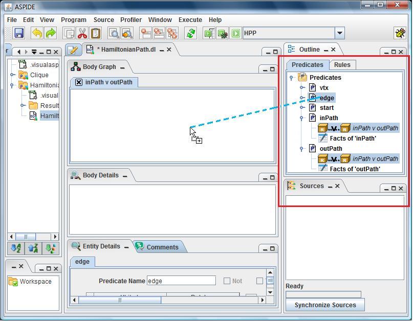
Figure 7. Outline with the disjunctive rule and dragging of the predicate edge in the Body Graph

A box representing the just added body predicate appears in the Body Graph and by clicking on the Link button to the first attribute of predicate edge, a pop-up menu allows for rapidly joining body and head (fig. 8).

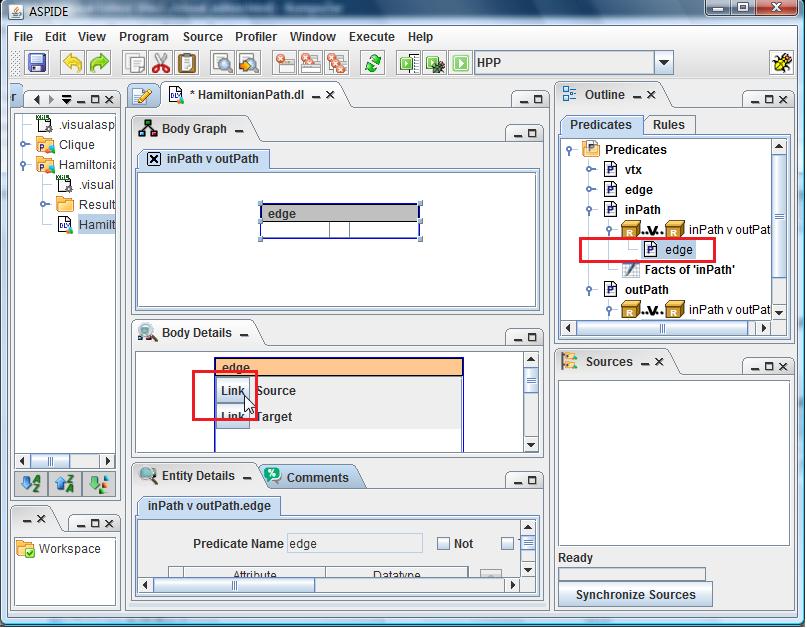
Figure 8. Dragged the predicate edge in the Body Graph. In the Outline the predicate edge
is added as child of the disjunctive rule node

In this case the predicates inPath and outPath have no attributes, so we will select New Attribute on the pop-up menu and the system will create a new attribute both in inPath and outPath making the projections. We do the same action also for the second attribute of edge (fig. 9). In the figure we can see, in the Entity Details the information regarding the projection; here we have already projected the attribute Source of edge and the head shows a new attribute Source for both inPath and outPath with the attribute bindings. The Body Graph and the Body Details show also the projection information.

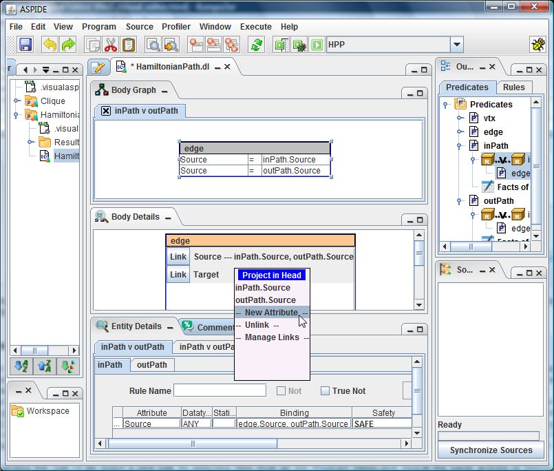
Figure 9. Projecting the attribute Target of the predicate edge.

Drawing Rules r2 and r3

The rule r2 contains two literals sharing variables. We insert a new rule by selecting New Rule on the Program menu; we name its head predicate reached. After that we select the predicate reached in the Outline and, using the Entity Details panel, we add a new attribute to the predicate reached naming it Node (fig. 10).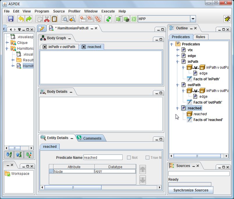

Figure 10. Created new rule with the predicate reached in head and added the attribute Node to the predicate

Now we drag in the body panel of the new rule, the predicates inPath and reached; note that this definition is recursive. Then, we join the two body literals by selecting both of them (this is done by clicking on the corresponding boxes in the body panel while pressing the shift key) and clicking on the join icon that appears on the top left of the selected boxes (fig. 11).

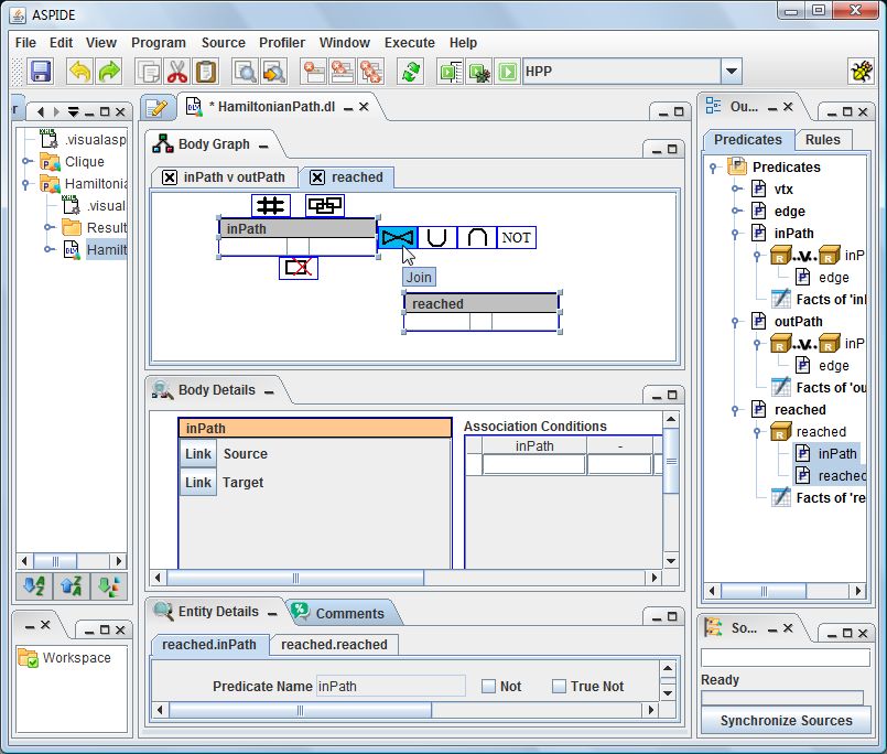
Figure 11. Join the predicates inPath e reached

The system will show a dialog window where one can setup the join (fig. 12). The details of the join are reported in the Body Details panel (fig. 13), where the joined attributes can further modified. As before, we properly link head and body attributes, in this case by acting on the link button corresponding to the second attribute of inPath.

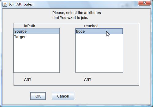
Figure 12. Join the attribute Target of the predicate inPath
and Node of the predicate reached.

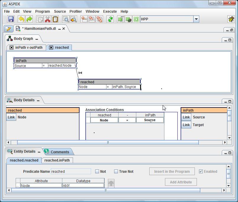
Figure 13. Details of the join

Regarding the rule r3 we insert a new rule by selecting New Rule on the Program menu and repeat the same actions of before by dragging of the predicate start and making the projection on head (fig. 14).

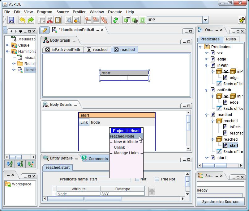
Project the attribute of the predicate start

Figure 14. Projection of the attribute Node of the predicate start in the head

Drawing Constraints r4 and r5

To create the constraint defined by the rule r4 we select New Constraint from the Program menu. The constraint, having a “forbidden” icon, appears on the Outline panel. The body of constraints can be specified in the same way as the body of rules i.e. by dragging predicates from the Outline panel. In our case we drag vtx and reached and make a join between the two predicates (fig. 15).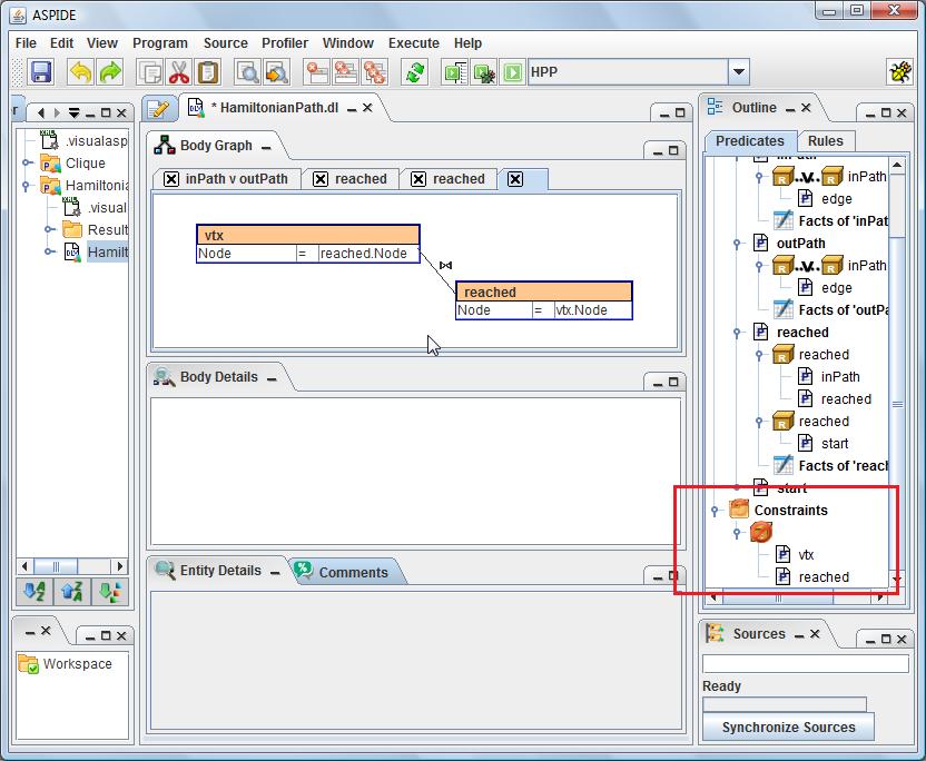

Figure 15. Created a new constraint and made a join between the predicates vtx and reached inserted in the body

To negate the predicate reached of the body, we select that predicate in the Body Graph panel and, on the Entity Details panel, we tick the checkbox Not and the predicate will become negated; in the Body Graph panel, the join arc between the two predicates will become an arrow from the predicate vtx to the negated predicate reached, the colour of the negated predicate will become different and, in the Outline panel, in the predicate name of reached the key word "not" will be added (fig. 16).

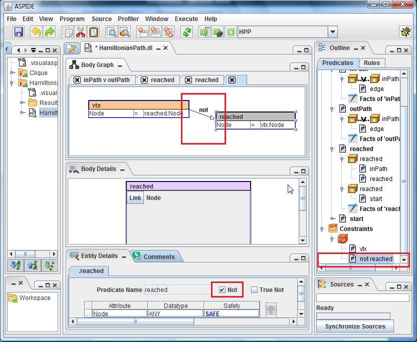
Figure 16. Negation of the predicate reached

The rule r5 is build using the same way of before.

Drawing Constraints r6 and r7

Both the constraints r6 and r7 contain an aggregate operator Count.

For r6 we create a new constraint as before, drag the predicates vtx and inPath and join the two predicates (fig. 17).

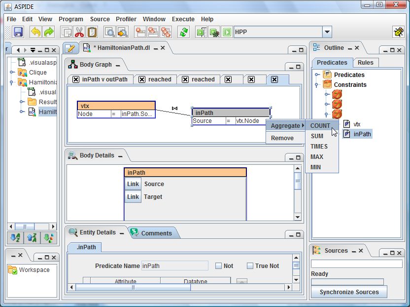
Figure 17. Aggregation of the predicate inPath

To aggregate the information contained in the predicate inPath we select that predicate in the body of the constraint and, with a right-click, we click on Aggregate and select Count from a drop-down menu (fig. 17). The result, shown in figure 18, is the specification of that new constraint.
In the Outline panel, the aggregate will be added and in the Body Graph panel a new entity with the aggregate will be created.
Note that, in the Body Details panel, an aggregate-specific box allows for setting guards, local variables etc.

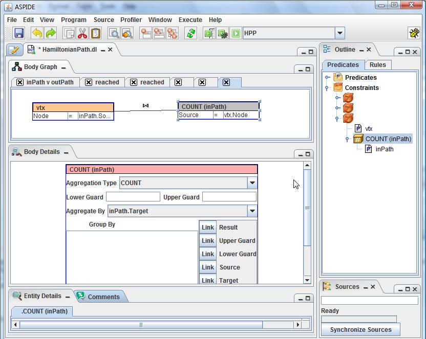
Figure 18. Result of the aggregation of the predicate inPath

At this point we repeat the same procedure to insert the constraint r7.

Switching from Visual Mode to Textual Mode

The program that we have just build graphically can be switched from visual mode to textual mode by clicking of the button Switch text/visual icon Switch Icon

available in the toolbar, and ASPIDE will show, in textual mode, the program built (fig. 19).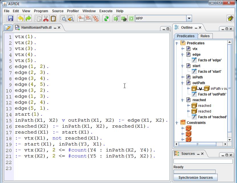

Figure 19. Textual view of the program built graphically.

Run Configuration

ASPIDE provides an advanced windows to configure the projects execution. A run configuration can include internal DLV files or external files, deciding the solver and option of execution to pass it at the moment of execution. The system automatically saves the used run configurations organazing them for project membership. The user can also choose whether to display the output of execution text mode or using the specific graphic interface.
Using the Run Configuration the users can have a single execution of the logic programs. The Run Configuration dialog is visible using the menu Execute - Show Run Configuration.